Example questions for Exam 3
Short answer
- Is it better to take many small samples or a few large samples? Why?
- What happens to confidence intervals as the sample size increases? Why?
- What is the difference between a population parameter and a sample statistic?
- What is a census?
- How do we know if a sample is good?
- Under what conditions can we use samples to generalize about the whole population?
Sampling and confidence intervals
- What does a confidence interval measure? Why is it useful?
- How can you narrow the width of a confidence interval?
A nonprofit executive director wants to know the average age of the volunteers her organization has used over the past year. She takes a random sample of 300 volunteers and uses bootstrapping-based simulation to construct a 95% confidence interval around the average. The sample average is 28.5 years old, and the confidence interval ranges between 20.3 and 33.4 years old. Which of the following are true?
- There’s a 95% chance that the true mean is between 20.3 and 33.4 years.
- 95% of the volunteers in the population are aged between 20.3 and 33.4 years.
- If the director took another random sample of 300 volunteers, there’s a 95% chance that the new mean would be between 20.3 and 33.4 years.
- She is 95% confidence that the interval between 20.3 and 33.4 years caputred the true population-level mean value.
- 95% of the volunteers responded to the executive director’s survey.
Hypothesis testing
Home values in Idaho and Arizona
## Setting `type = "permute"` in `generate()`.You collect data about average county-level home values in Idaho and Arizona and you want to know if houses tend to be more expensive in one of the states. You calculate that the average home value in Arizona is $22,378.48 higher than in Idaho. You want to test to make sure that difference really is positive.
Through simulation, you determine that the distribution of the between-state differences in a hypothetical world where there’s no difference looks like the histogram below. The actual sample difference of $22,378.48 is marked in red. The associated p-value is 0.0976.
## Warning: `visualize()` shouldn't be used to plot p-value. Arguments
## `obs_stat`, `obs_stat_color`, `pvalue_fill`, and `direction` are
## deprecated. Use `shade_p_value()` instead.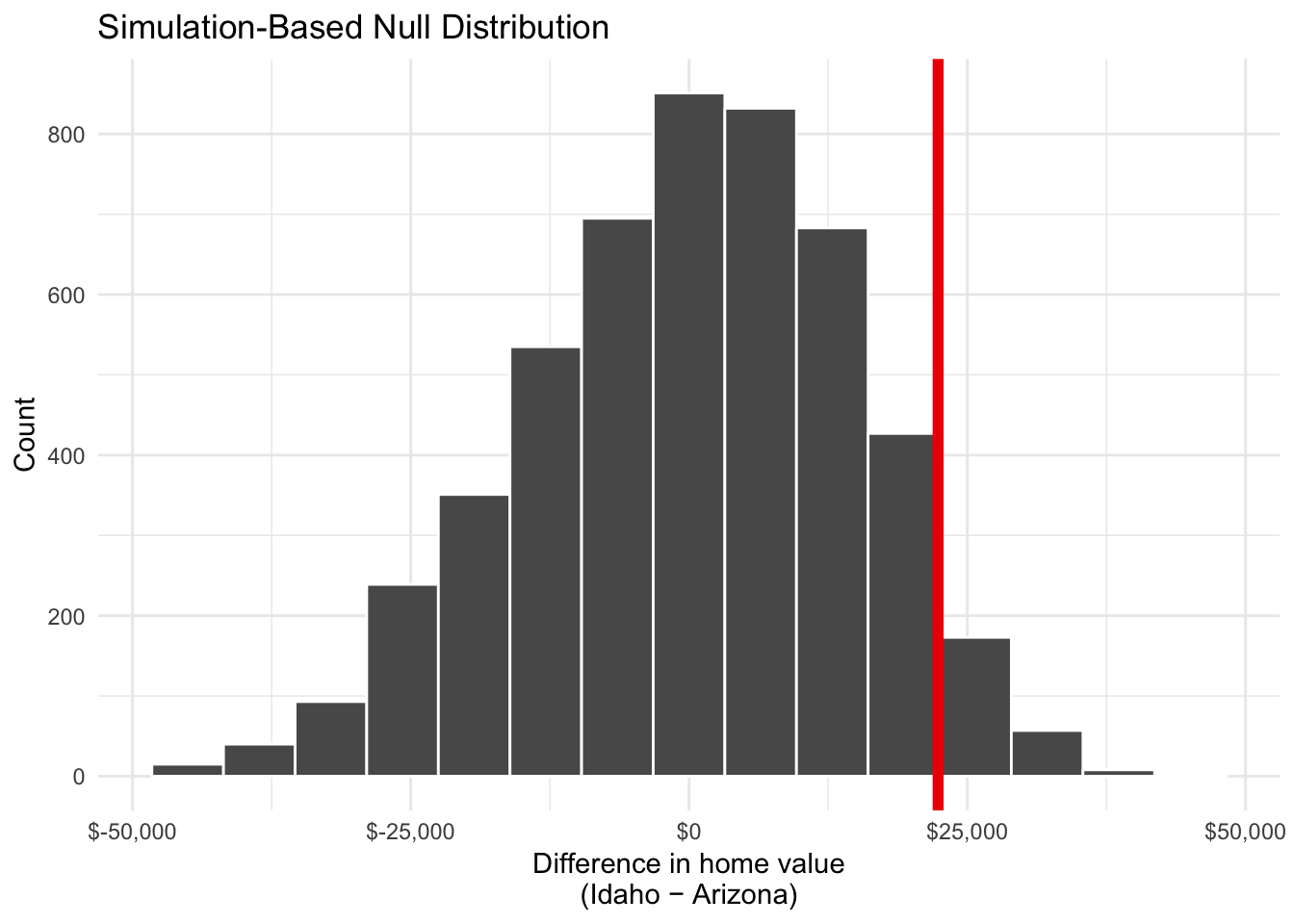
- What is your null hypothesis?
- What is your alternative hypothesis?
- What can you conclude about the difference between the two groups?
Conservatives and kids
## Setting `type = "permute"` in `generate()`.You use data from the 2016 General Social Survey (GSS) to investigate the relationship between political ideology and the number of children people have. Based on a sample of 2,867 people, you find that self-reported conservatives have an average of 2.03 children, while those who are not conservative (i.e. those who are neutral or liberal) have an average of 1.68 children. The difference between these two averages is -0.35.
Through simulation, you determine that the distribution of the difference in the average number of kids between these two groups looks like the histogram below. The actual sample difference is marked in red. The associated p-value is 0 (or < 0.001).
## Warning: `visualize()` shouldn't be used to plot p-value. Arguments
## `obs_stat`, `obs_stat_color`, `pvalue_fill`, and `direction` are
## deprecated. Use `shade_p_value()` instead.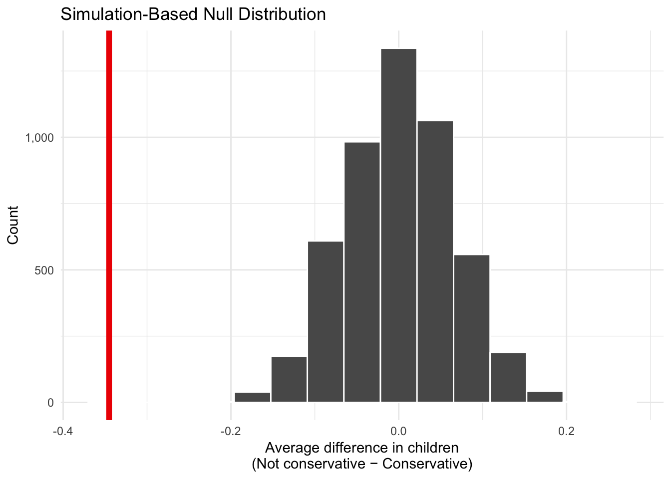
- What is your null hypothesis?
- What is your alternative hypothesis?
- What can you conclude about the difference between the two groups?
Marital status and presidential elections
## Setting `type = "permute"` in `generate()`.You use data from the 2016 General Social Survey (GSS) to investigate the relationship between marital status and 2012 presidential election results. Based on a sample of 2,867 people, you find that 40.2% of those who voted for Barack Obama in 2012 were married, compared to 57.9% of those who voted for Mitt Romney. The difference between these two proportions is 17.7%.
Through simulation, you determine that the distribution of the possible differences in the proportion of married people who voted for Obama and Romney looks like the histogram below. The actual sample difference is marked in red. The associated p-value is 0 (or < 0.001).
## Warning: `visualize()` shouldn't be used to plot p-value. Arguments
## `obs_stat`, `obs_stat_color`, `pvalue_fill`, and `direction` are
## deprecated. Use `shade_p_value()` instead.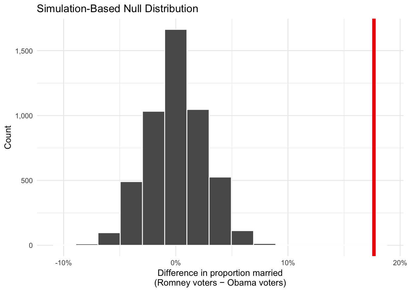
- What is your null hypothesis?
- What is your alternative hypothesis?
- What can you conclude about the difference between the two groups?
Inference and regression
There will be 1–2 short regression tables to interpret. In the past you’ve only looked at the estimate column. This time you’ll need to interpret the estimate column and consider the coefficient’s statistical significance.
We use the following multiple regression model to predict/explain property taxes in the Western United States.
\[ \begin{aligned} \hat{\text{tax per housing unit}} =& \beta_0 + \beta_1 \text{median home value} + \beta_2 \text{proportion of houses with kids } + \\ & \beta_3 \text{California} + \beta_4 \text{Idaho} + \beta_4 \text{Nevada} + \beta_6 \text{Utah} + \epsilon \end{aligned} \]
This model provides us with the following results:
| term | estimate | std_error | statistic | p_value | lower_ci | upper_ci |
|---|---|---|---|---|---|---|
| intercept | -412.5 | 118.1 | -3.493 | 0.001 | -645.8 | -179.2 |
| median_home_value | 0.004 | 0 | 21.99 | 0 | 0.004 | 0.004 |
| prop_houses_with_kids | 14.09 | 2.853 | 4.941 | 0 | 8.459 | 19.73 |
| stateCalifornia | 123.3 | 88.22 | 1.397 | 0.164 | -50.98 | 297.5 |
| stateIdaho | 9.526 | 82.74 | 0.115 | 0.908 | -153.9 | 173 |
| stateNevada | 102.5 | 98.25 | 1.043 | 0.299 | -91.63 | 296.5 |
| stateUtah | -213.2 | 91.21 | -2.337 | 0.021 | -393.3 | -33.03 |
Interpret the following coefficients and include an interpretation of the p-value and/or confidence interval. Is the coefficient significantly different from zero?
median_home_valueprop_houses_with_kidsstateCaliforniastateIdahostateNevadastateUtah