Example questions for Exam 2
Short answer
- What is the difference between \(R^2\) and adjusted \(R^2\)?
- How do we know what the best fit of a regression line is?
- What does it mean to account for other variables in a regression model?
- What does it mean when we say that the coefficients for categorical variables are not slopes?
Correlation
Coefficients
Interpret the following correlation coefficients:
- 0.64
- 0.11
- -0.92
- -0.01
- 0.39
Scatterplots
Guess a correlation coefficient for each of these plots:
## Warning: `as_tibble.matrix()` requires a matrix with column names or a `.name_repair` argument. Using compatibility `.name_repair`.
## This warning is displayed once per session.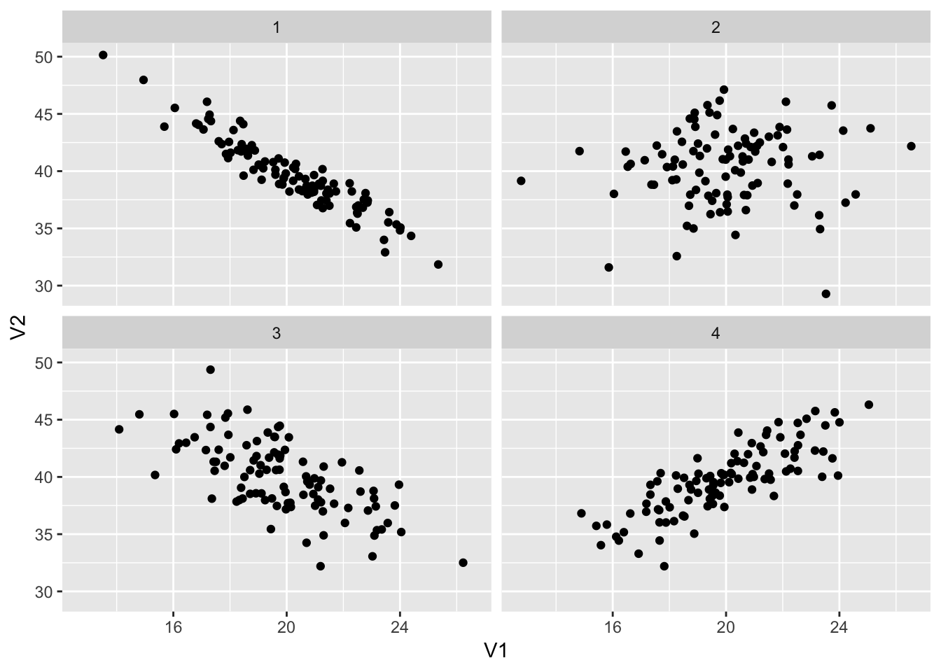
- Plot 1
- Plot 2
- Plot 3
- Plot 4
Multiple regression
There will be two questions structured similarly to this one, but with different emphases (i.e. just interpreting coefficients, just interpreting \(R^2\), etc.).
You come across a data set with information about every Nintento Wii Mario Kart game listing on eBay in October 2009. There are 141 rows, each representing one eBay posting. There are columns indicating many different variables:
price: The final price of the gameduration: The number of days the game was listed on eBayused: A categorical variable indicating if the game was new or used (base case = “new”)num_bids: The number of bids made during the auctionseller_rating: The number of ratings the seller has on eBayhas_photo: A categorical variable indicating if the seller included a stock photograph of the game (base case = “no”)num_wheels: The number of Wii wheel controllers included with the game
Variable identification
We are interested in predicting the final price of a Mario Kart game sold on eBay, based on a host of factors. We run the following multiple regression model:
\[ \begin{align} \text{Model 1: } \widehat{\text{price}} &= \beta_0 + \beta_1 \text{duration} + \beta_2 \text{num_bids} + \beta_3 \text{used} + \\ &\beta_4 \text{seller_rating} + \beta_5 \text{has_photo} + \beta_6 \text{duration} \end{align} \]
- What is/are the outcome (or dependent) variable(s)?
- What is/are the explanatory (or independent) variable(s)?
Interpreting output
Here is the output from this regression model:
model1 <- lm(price ~ duration + num_bids + used +
               seller_rating + has_photo + num_wheels,
             data = mario_kart)
model1 %>% get_regression_table()
## # A tibble: 7 x 7
## term estimate std_error statistic p_value lower_ci upper_ci
## <chr> <dbl> <dbl> <dbl> <dbl> <dbl> <dbl>
## 1 intercept 40.8 2.04 20.0 0 36.8 44.9
## 2 duration 0.035 0.184 0.192 0.848 -0.328 0.399
## 3 num_bids -0.066 0.071 -0.932 0.353 -0.207 0.074
## 4 usedused -4.62 1.02 -4.54 0 -6.63 -2.61
## 5 seller_rating 0 0 3.64 0 0 0
## 6 has_photoyes 0.968 1.01 0.957 0.34 -1.03 2.97
## 7 num_wheels 7.72 0.553 13.9 0 6.62 8.81Interpret the following coefficients (remember the template!):
duration
num_bids
used
num_wheels
Interpreting fit
The following code shows a summary of the model diagnostics:
model1 %>% get_regression_summaries()## # A tibble: 1 x 8
## r_squared adj_r_squared mse rmse sigma statistic p_value df
## <dbl> <dbl> <dbl> <dbl> <dbl> <dbl> <dbl> <dbl>
## 1 0.749 0.737 20.7 4.55 4.67 66.5 0 7- How much variation in final price does this model explain?
Comparing models
After running this first model, you run a couple simpler models that predict price based on whether the game is used, and one based on whether the game is used, how long it’s posted, and how many wheel controllers are included:
\[ \begin{align} \text{Model 2: }\widehat{\text{price}} &= \beta_0 + \beta_1 \text{used} \end{align} \]
\[ \begin{align} \text{Model 3: }\widehat{\text{price}} &= \beta_0 + \beta_1 \text{used} + \beta_2 \text{duration} + \beta_3 \text{num_wheels} \end{align} \]
This table provides the \(R^2\) and adjusted \(R^2\) values for the three models.
| model | formula | r.squared | adj.r.squared |
|---|---|---|---|
| Model 1 | price ~ duration + num_bids + used + seller_rating + has_photo + num_wheels | 0.7487 | 0.7375 |
| Model 2 | price ~ used | 0.3506 | 0.3459 |
| Model 3 | price ~ used + duration + num_wheels | 0.7169 | 0.7107 |
- Which of these models explains the most variation in price? How much variation does it explain?