Bootstrapping and confidence intervals
Materials for class on Thursday, November 8, 2018
Contents
Slides
Download the slides from today’s lecture:

Bootstrap reporting form
Go here to report your bootstrap median:
Live code
Use this link to see the code that I’m actually typing:
I’ve saved the R script to Dropbox, and that link goes to a live version of that file. Refresh or re-open the link as needed to copy/paste code I type up on the screen.
Bootstrapping with R
In class we used the rents of 20 randomly selected apartments in Manhattan to explore how bootstrapping works. Here’s how to do that exploration in R. Load these packages to get started, and download these two datasets (and put them in a folder named “data”):
library(tidyverse)
library(moderndive)
library(infer)
library(scales)

# Setting a random seed ensures that every random draw will be the same each
# time you run this (and regardless of what computer you run this on)
set.seed(1234)
manhattan <- read_csv("data/manhattan.csv")
class_rent_boot <- read_csv("data/class_rent_boot.csv")In-class results
In class, we were interested in the true population-level median 1-bedroom Manhattan apartment rent. This is our unmeasurable population parameter. The only way to get close to it is through sampling and statistics—we can calculate the sample median and calculate a confidence interval for that median to determine how big of a net we have and how confident we are that our confidence interval captured the population parameter.
First, we can look at the sample median. This has nothing to do with bootstrapping yet—this is just the median value of the 20 random apartments.
sample_median <- manhattan %>%
  summarize(stat = median(rent))
sample_median
## # A tibble: 1 x 1
## stat
## <dbl>
## 1 2350The median rental price is $2,350 a month. Here’s what the distribution of rents from our sample looks like, with the median price overlaid with geom_vline():
ggplot(manhattan, aes(x = rent)) +
  geom_histogram(binwidth = 250, color = "white") +
  geom_vline(xintercept = sample_median$stat, color = "red", size = 1) +
  scale_x_continuous(labels = dollar) +
  labs(x = "Rent", y = "Count",
       caption = "Sample median in red")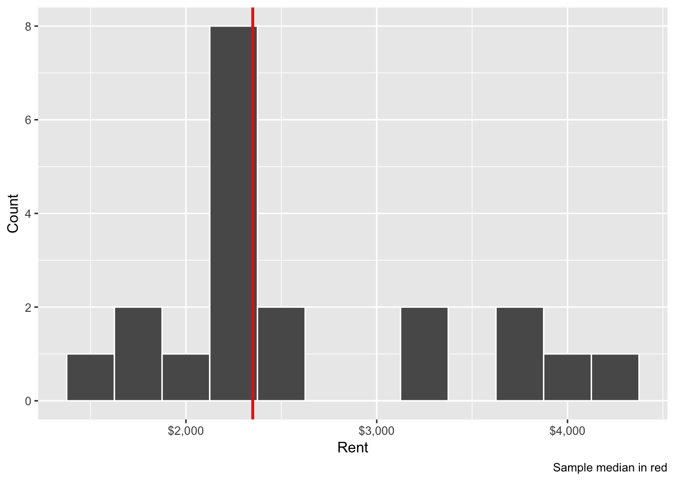
How confident are we with this sample median? Is that really representative of the true population parameter? Some of these apartments are under $2,000; some are above $4,000. Is this median really typical?
We can measure our confidence by building a confidence interval for our median, which will allow us to make better inference about the whole population of Manhattan apartments. We can calculate confidence intervals in two ways: math and simulation. We’ll use simulation this week (bootstrapping) and math later on.
In class, you all did a manual bootstrapping process. You took a single sample from our sample of 20 apartments, wrote down the number, replaced the paper, and drew another sample until you had a new bootstrapped sample with 20 observations. Some of these 20 were repeated, which is by design.
You then calculated the median of your bootstrap sample and we made a histogram on the board. Here’s the ggplot version of that histogram, with the sample median marked in red again:
ggplot(class_rent_boot, aes(x = rent)) +
  geom_histogram(binwidth = 100, color = "white") +
  geom_vline(xintercept = sample_median$stat, color = "red", size = 1) +
  scale_x_continuous(labels = dollar) +
  labs(x = "Rent", y = "Count",
       caption = "35 bootstrapped medians; sample median in red")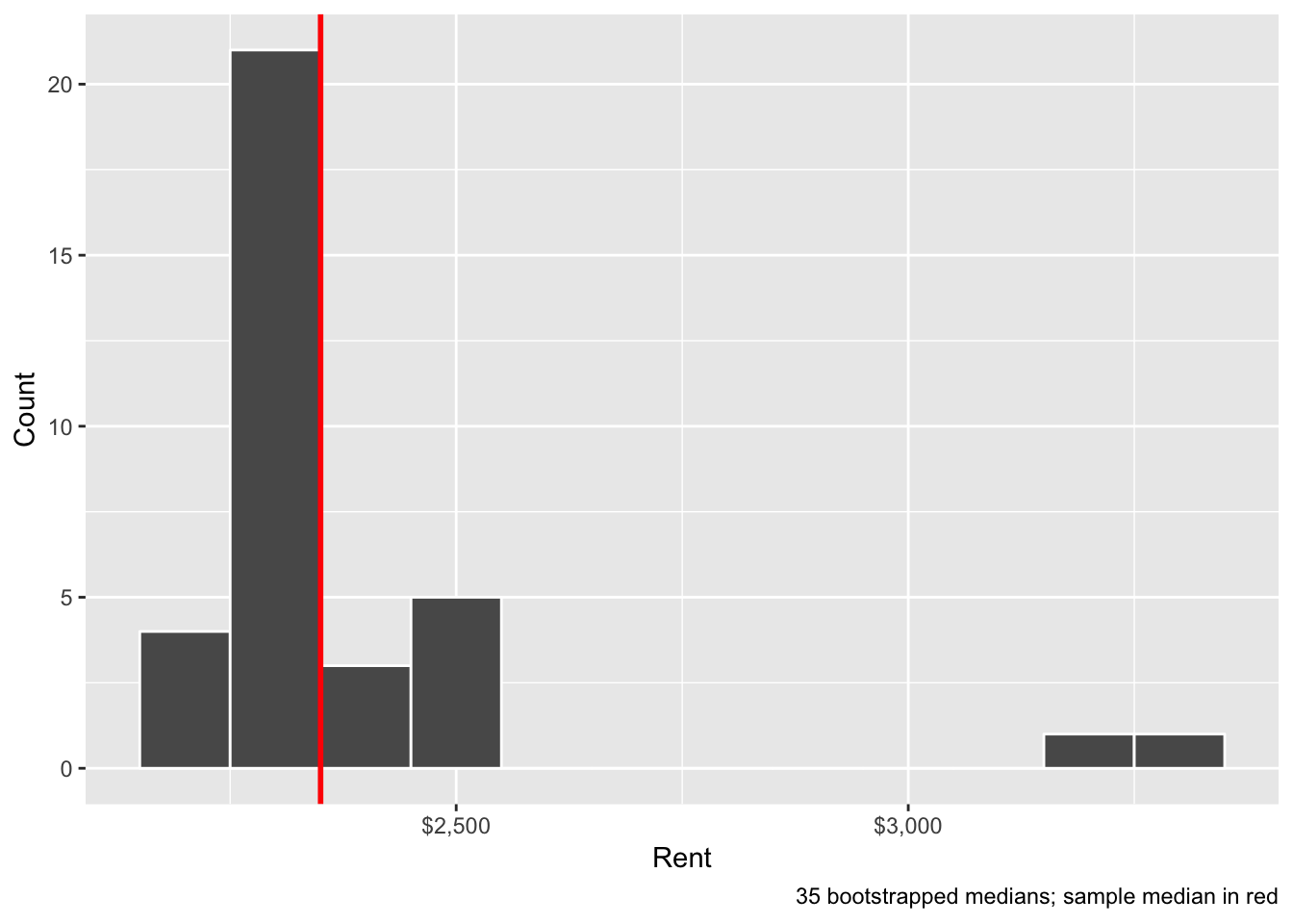
To find the 95% confidence interval, we need to find the middle 95% of this distribution, or the range from the 2.5% percentile to the 97.5% percentile. We can do this with the quantile() function:
class_rent_ci <- class_rent_boot %>%
  summarize(lower = quantile(rent, 0.025),
            upper = quantile(rent, 0.975))
class_rent_ci
## # A tibble: 1 x 2
## lower upper
## <dbl> <dbl>
## 1 2171. 3210.This range means that the 95% confidence interval of rents in Manhattan, based on 35 bootstrapped samples, is ($2,171, $3,210). We are 95% confident that this net captures the true population median.
Bootstrapping with R and infer
That’s a pretty wide interval though, and we can get a better estimate of the variation in the sample by taking more bootstrapped samples. Instead of 35 manual samples, we can take 1,000 automated samples of the original 20 Manhattan apartments using the infer library.
The standard usage of infer is to specify() the column(s) we’re interested in, generate() a bunch of simulated data based on that column, and then calculate() a sample statistic for the simulated data:
boot_rent <- manhattan %>%
  # Specify the variable of interest
  specify(response = rent) %>%
  # specify(rent ~ NULL)  # This does the same thing
  # Generate a bunch of bootstrap samples
  generate(reps = 1000, type = "bootstrap") %>%
  # Find the median of each sample
  calculate(stat = "median")

# See the first few rows
head(boot_rent)
## # A tibble: 6 x 2
## replicate stat
## <int> <dbl>
## 1 1 2350
## 2 2 2350
## 3 3 2350
## 4 4 2550
## 5 5 2350
## 6 6 2350We can visualize this with a histogram. This is the same as the in-class histogram above, only now this is based on the medians of 1,000 bootstrapped distributions instead of 35:
ggplot(boot_rent, aes(x = stat)) +
  geom_histogram(binwidth = 100, color = "white") +
  geom_vline(xintercept = sample_median$stat, color = "red", size = 1) +
  scale_x_continuous(labels = dollar) +
  labs(x = "Rent", y = "Count",
       caption = "1,000 bootstrapped medians; sample median in red")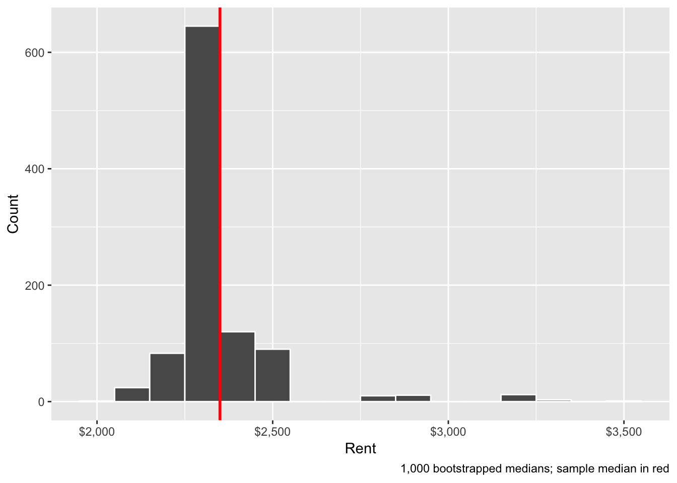
Or, instead of using regular ggplot, we can use the visualize() function from infer, which is just a fancy wrapper for ggplot:
boot_rent %>%
  visualize(obs_stat = sample_median$stat, obs_stat_color = "red") +
  scale_x_continuous(labels = dollar) +
  labs(x = "Rent", y = "Count",
       caption = "1,000 bootstrapped medians; sample median in red")
## Warning: `visualize()` shouldn't be used to plot p-value. Arguments
## `obs_stat`, `obs_stat_color`, `pvalue_fill`, and `direction` are
## deprecated. Use `shade_p_value()` instead.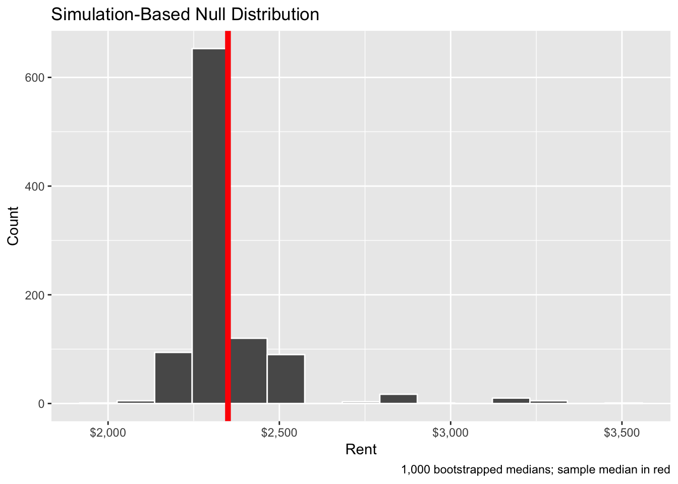
We can then find the 95% confidence interval for this distribution with the get_ci() function from infer:
boot_rent_ci <- boot_rent %>%
  get_ci(level = 0.95, type = "percentile")
boot_rent_ci
## # A tibble: 1 x 2
## `2.5%` `97.5%`
## <dbl> <dbl>
## 1 2160. 2875This range means that the 95% confidence interval of rents in Manhattan, based on 1,000 bootstrapped samples from our original 20-apartment sample, is ($2,160, $2,875). We are 95% confident that this net captures the true population median. The lower part of that range is about the same as our by-hand version, but the upper part is considerably smaller.
We can plot this confidence interval in two ways. First, the visualize() way:
boot_rent %>%
  visualize(endpoints = boot_rent_ci, direction = "between") +
  scale_x_continuous(labels = dollar) +
  labs(x = "Rent", y = "Count",
       caption = "1,000 bootstrapped medians; 95% confidence interval in green")
## Warning: `visualize()` shouldn't be used to plot confidence interval.
## Arguments `endpoints`, `endpoints_color`, and `ci_fill` are deprecated. Use
## `shade_confidence_interval()` instead.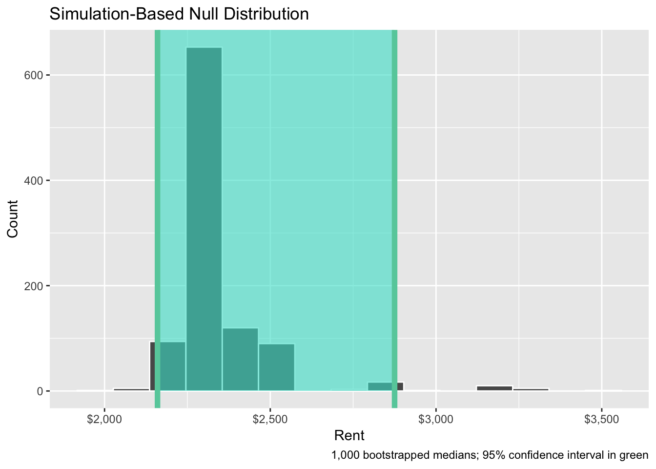
Or the regular ggplot way:
ggplot(boot_rent, aes(x = stat)) +
  annotate(geom = "rect", xmin = boot_rent_ci$`2.5%`, xmax = boot_rent_ci$`97.5%`,
           ymin = -Inf, ymax = Inf, alpha = 0.5, fill = "turquoise") +
  geom_histogram(binwidth = 100, color = "white") +
  geom_vline(xintercept = boot_rent_ci$`2.5%`, color = "mediumaquamarine", size = 2) +
  geom_vline(xintercept = boot_rent_ci$`97.5%`, color = "mediumaquamarine", size = 2) +
  geom_vline(xintercept = sample_median$stat, color = "red", size = 1) +
  scale_x_continuous(labels = dollar) +
  labs(x = "Rent", y = "Count",
       caption = "1,000 bootstrapped medians; sample median in red; 95% confidence interval in green")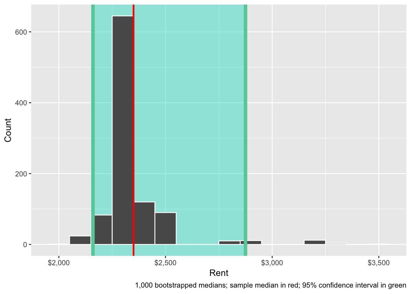
Clearest and muddiest things
Go to this form and answer these three questions:
- What was the muddiest thing from class today? What are you still wondering about?
- What was the clearest thing from class today?
- What was the most exciting thing you learned?
I’ll compile the questions and send out answers after class.