Multiple regression
Materials for class on Thursday, October 18, 2018
Contents
Slides
Download the slides from today’s lecture:

Predicting temperature
At the end of class today, we looked at the factors that predict the daily high temperature in Provo (specifically 40.248752, -111.649216) from January to May 2017. Here’s a cleaner version of that analysis.
Load and wrangle data
First, we load the libraries we’ll be using:
library(tidyverse)
library(lubridate)
library(moderndive)
library(scales)  # For nicer axis labels
Then we load the data. I used the darksky R package to download this historical data from Dark Sky, and then I saved the CSV file online.
# This reads the CSV file directly from the internet
weather_provo_raw <- read_csv("https://andhs.co/provoweather")
Then we clean and wrangle the data, or make adjustments to it so that it’s easier to use and model and plot. I include comments explaining what each line does below:
weather_provo_2017 <- weather_provo_raw %>%
         # Extract the month name from the date
  mutate(month = month(date, label = TRUE, abbr = FALSE),
         # Extract the month number from the date
         month_number = month(date, label = FALSE),
         # Extract the day of the week from the date
         weekday = wday(date, label = TRUE, abbr = FALSE),
         # Extract the number of the day of the week (1 = Sunday)
         weekday_number = wday(date, label = FALSE)) %>%
  # Change all the missing values in the precipType column to "none"
  mutate(precipType = ifelse(is.na(precipType), "none", precipType)) %>%
  # Only select these columns
  select(date, month, month_number, weekday, weekday_number,
         sunriseTime, sunsetTime, moonPhase, precipProbability, precipType,
         temperatureHigh, temperatureLow, dewPoint, humidity, pressure,
         windSpeed, cloudCover, visibility, uvIndex)

# Make a subset of the clean data that only includes January through May
winter_spring <- weather_provo_2017 %>%
  filter(month_number <= 5) %>%
  # After we filter, R still thinks that the month column has 12 possible
  # categories. Here, we tell it to be a factor again (it already is one) so
  # that it only includes January through May
  mutate(month = factor(month, ordered = FALSE)) %>%
  # Finally, we multiply some of the percentage variables by 100 so the
  # regression coefficients are easier to interpret
  mutate(humidity = humidity * 100,
         cloudCover = cloudCover * 100,
         precipProbability = precipProbability * 100)
Explore data
First we can look at how the high temperature changed over time. Not surprisingly, it went up.
ggplot(winter_spring, aes(x = date, y = temperatureHigh)) +
  geom_line() +
  geom_smooth(method = "lm", se = FALSE) +
  scale_y_continuous(labels = degree_format()) +
  labs(x = NULL, y = "High temperature") +
  theme_minimal()
Next we look at how humidity has changed over time. It went down:
ggplot(winter_spring, aes(x = date, y = humidity)) +
  geom_line() +
  geom_smooth(method = "lm", se = FALSE) +
  labs(x = NULL, y = "Humidity") +
  theme_minimal()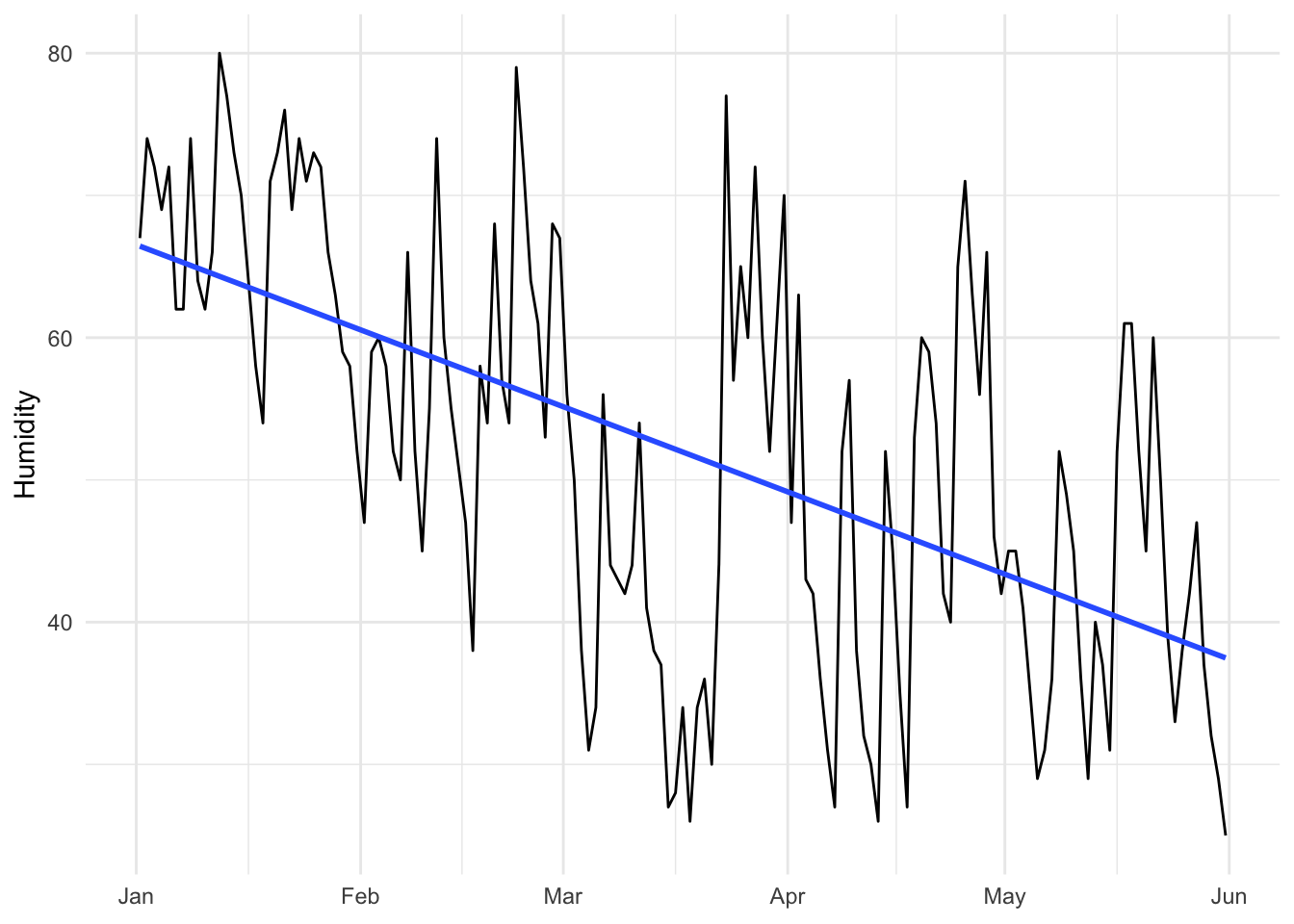
Neat.
Humidity and temperature
Our main research question is exploring the relationship between humidity and temperature. Are they correlated, and if so, how much does temperature change as humidity increases or decreases?
Our outcome variable (or y or response or dependent variable) is thus temperatureHigh, while our main explanatory variable (or x or independent variable) is humidity.
First we check to see how correlated they are, both visually and with a correlation coefficient:
ggplot(winter_spring, aes(x = humidity, y = temperatureHigh)) +
  geom_point() +
  geom_smooth(method = "lm", se = FALSE) +
  scale_y_continuous(labels = degree_format()) +
  labs(x = "Humidity", y = "High temperature") +
  theme_minimal()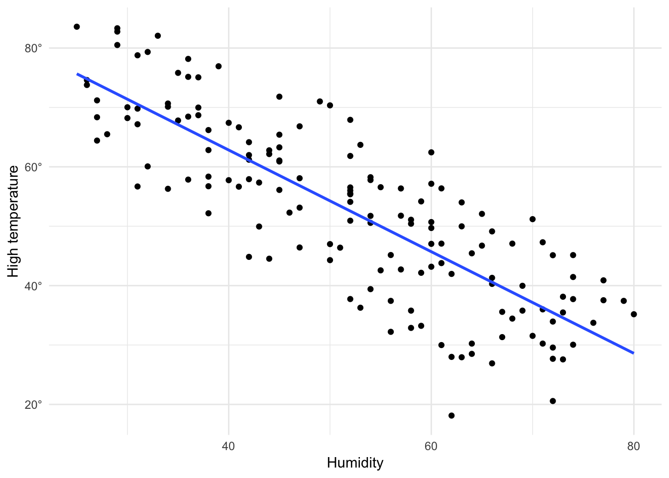
The graph shows that the two variables are definitely negatively correlated (as humidity increases, temperature decreases). The correlation between the two is…
winter_spring %>%
  get_correlation(temperatureHigh ~ humidity)
## # A tibble: 1 x 1
## correlation
## <dbl>
## 1 -0.821…-0.821. That’s close to 1, so we can say that temperature and humidity are strongly negatively correlated (r = -0.821).
Next, we want to see how much temperature changes as humidity changes. We use a linear model to find the slope and intercept of this line:
model1 <- lm(temperatureHigh ~ humidity, data = winter_spring)
model1 %>% get_regression_table()
## # A tibble: 2 x 7
## term estimate std_error statistic p_value lower_ci upper_ci
## <chr> <dbl> <dbl> <dbl> <dbl> <dbl> <dbl>
## 1 intercept 97.0 2.62 37.0 0 91.9 102.
## 2 humidity -0.856 0.049 -17.6 0 -0.952 -0.759First, we see if the intercept (\(\beta_0\)) provides helpful information. The intercept is 97, which means that on average, during the period of January to May 2017, if humidity was 0, the predicted temperature would be 97˚. That seems… really really high. There were 0 days with 0 humidity during this time period (the lowest humidity level was 25), so it’s a stretch to try to interpret this for non-existent extra-humid days. We can safely disregard the intercept.
The \(\beta_1\) coefficient, or slope of humidity, shows that for every 1 point increase in humidity, there is an associated drop in temperature of 0.856˚, on average. As the weather becomes more humid, the high daily temperature becomes colder. This is probably because humidity in the winter is a sign of snow—I’m guessing this relationship is reversed in summer months, where humidity leads to muggier weather.
Months and temperature
Next, we want to see what the effect of time is on temperature. While humidity explains some of the variation in temperature, from previous experience in being alive, we know that the weather naturally warms up as we approach summer, regardless of humidity or any other factor. We can see this if we look at the average temperature per month:
winter_spring %>%
  group_by(month) %>%
  summarize(avg_high = mean(temperatureHigh))
## # A tibble: 5 x 2
## month avg_high
## <fct> <dbl>
## 1 January 33.9
## 2 February 45.7
## 3 March 56.6
## 4 April 56.8
## 5 May 69.3Not surprisingly, January was really cold on average, while May was not. The other months fall somewhere in between.
If we include month in the regression model, we’ll get a coefficient for each month except the base case, which is the first category (January in this case):
model2 <- lm(temperatureHigh ~ month, data = winter_spring)
model2 %>% get_regression_table()
## # A tibble: 5 x 7
## term estimate std_error statistic p_value lower_ci upper_ci
## <chr> <dbl> <dbl> <dbl> <dbl> <dbl> <dbl>
## 1 intercept 33.9 1.65 20.5 0 30.6 37.2
## 2 monthFebruary 11.8 2.40 4.94 0 7.11 16.6
## 3 monthMarch 22.8 2.34 9.74 0 18.1 27.4
## 4 monthApril 22.9 2.35 9.75 0 18.3 27.6
## 5 monthMay 35.4 2.34 15.2 0 30.8 40.0These coefficients are not slopes. They are shifts in the intercept. Notice how the intercept is 33.9—identical to January’s average high temperature. All other month-based coefficients show the adjustment in average temperature per month using January as the base case. February is 11.8˚ warmer than January, on average. March is 22.8˚ warmer than January, on average. April is 22.9˚ warmer than January, on average. May is 35.4˚ warmer than January, on average.
Humidity, months, and temperature
Both humidity and month explain variation in temperatures. This is obvious in this scatterplot, which colors the points by month. Points for May are clustered in the top left corner, while points in January are clustered in the bottom right.
ggplot(winter_spring, aes(x = humidity, y = temperatureHigh)) +
  geom_point(aes(color = month)) +
  geom_smooth(method = "lm", se = FALSE) +
  scale_y_continuous(labels = degree_format()) +
  labs(x = "Humidity", y = "High temperature") +
  theme_minimal()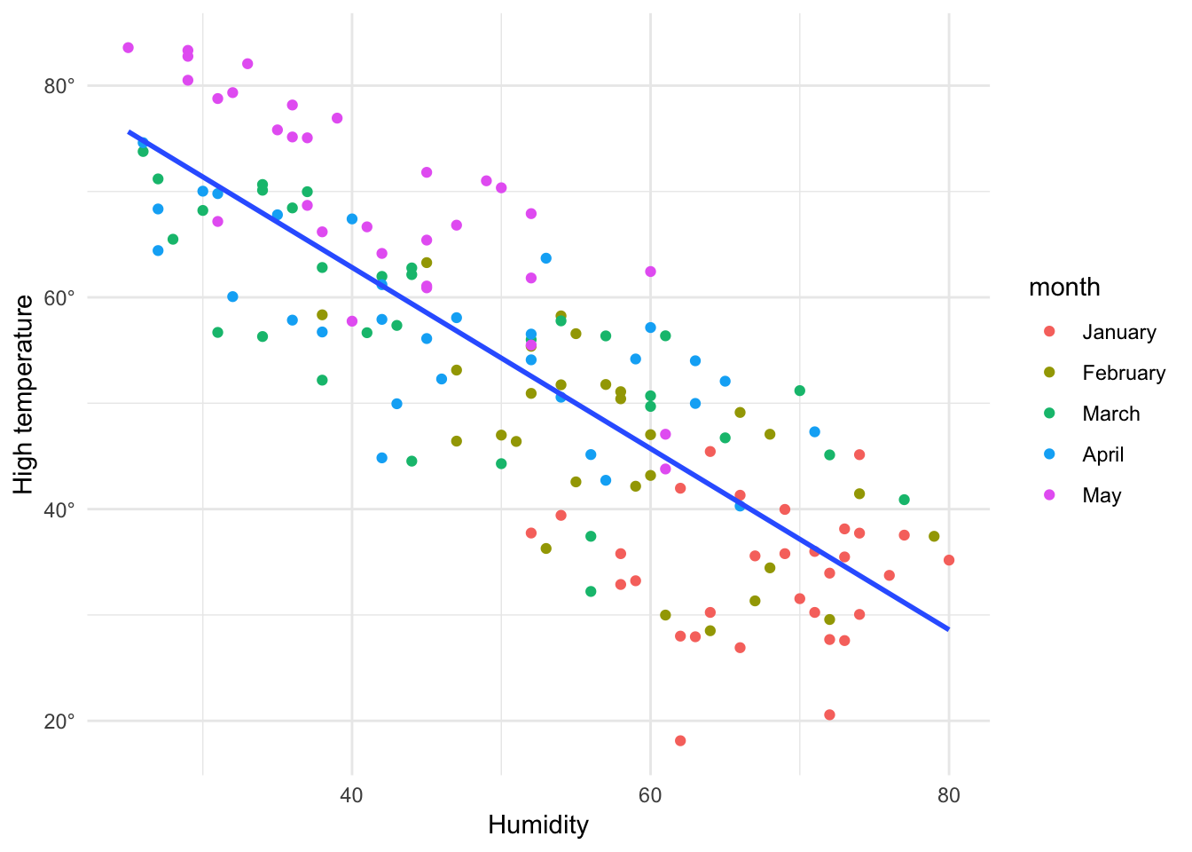
If we include both humidity and month in the model, we can get an estimate of the effect of humidity controlling for or taking into account time (or month).
model3 <- lm(temperatureHigh ~ humidity + month, data = winter_spring)
model3 %>% get_regression_table()
## # A tibble: 6 x 7
## term estimate std_error statistic p_value lower_ci upper_ci
## <chr> <dbl> <dbl> <dbl> <dbl> <dbl> <dbl>
## 1 intercept 71.8 3.70 19.4 0 64.5 79.1
## 2 humidity -0.56 0.052 -10.9 0 -0.662 -0.458
## 3 monthFebruary 6.44 1.85 3.48 0.001 2.78 10.1
## 4 monthMarch 10.9 2.05 5.30 0 6.83 15.0
## 5 monthApril 11.2 2.06 5.43 0 7.11 15.3
## 6 monthMay 20.7 2.20 9.39 0 16.3 25.1Now we have a slope for humidity, as well as several shifts in intercept based on month. We can start by interpreting the \(\beta_0\) coefficient. This shows the average temperature in January when humidity is at 0. 71˚ still seems really high for January, but recall that there are no days with 0 humidity, so it’s a stretch to try to get anything meaningful out of the intercept.
We can make the following statements about this model:
- Controlling for month, a one point increase in humidity is associated with a 0.56˚ drop in temperature, on average.
- Controlling for humidity, the high temperature in February is 6.4˚ warmer than in January, on average. Note that this is a lot different than the \(\beta\) from the previous model (there it was 11.8). That’s because humidity is now explaining some of the variation in temperature.
- Controlling for humidity, the high temperature in March is 10.9˚ warmer than in January, on average.
- Taking humidity into account, the high temperature in April is 11.2˚ warmer than in January, on average.
- On average, if we take humidity into account, the high temperature in May is 20.7˚ higher than in January.
Humidity, wind, and clouds
For fun, we can see what the effect of other weather-related variables is on high temperature. Here we build a model using humidity, wind speed, and cloud cover to explain variation in temperature.
model4 <- lm(temperatureHigh ~ humidity + windSpeed + cloudCover,
             data = winter_spring)
model4 %>% get_regression_table()
## # A tibble: 4 x 7
## term estimate std_error statistic p_value lower_ci upper_ci
## <chr> <dbl> <dbl> <dbl> <dbl> <dbl> <dbl>
## 1 intercept 103. 3.67 28.0 0 95.5 110.
## 2 humidity -0.992 0.08 -12.4 0 -1.15 -0.833
## 3 windSpeed -0.959 0.533 -1.80 0.074 -2.01 0.093
## 4 cloudCover 0.074 0.036 2.04 0.043 0.002 0.146We can make the following statements:
- Controlling for wind speed and cloud cover, a one unit increase in humidity is associated with a 0.992˚ lower temperature, on average.
- Taking humidity and cloud cover into account, a 1 MPH increase in wind speed is associated with a lower temperature of 0.959˚, on average.
- On average, controlling for humidity and wind speed, a one percent increase in cloud cover is associated wig a higher temperature of 0.074˚.
Humidity, wind, clouds, and month
We can also account for month when looking at humidity, wind speed, and cloud cover:
model5 <- lm(temperatureHigh ~ humidity + windSpeed + cloudCover + month,
             data = winter_spring)
model5 %>% get_regression_table()
## # A tibble: 8 x 7
## term estimate std_error statistic p_value lower_ci upper_ci
## <chr> <dbl> <dbl> <dbl> <dbl> <dbl> <dbl>
## 1 intercept 74.5 4.41 16.9 0 65.7 83.2
## 2 humidity -0.658 0.074 -8.85 0 -0.805 -0.511
## 3 windSpeed -0.101 0.438 -0.231 0.817 -0.967 0.764
## 4 cloudCover 0.06 0.029 2.07 0.04 0.003 0.117
## 5 monthFebruary 6.14 1.85 3.33 0.001 2.49 9.79
## 6 monthMarch 10.7 2.04 5.23 0 6.63 14.7
## 7 monthApril 11.1 2.04 5.43 0 7.04 15.1
## 8 monthMay 20.8 2.21 9.40 0 16.4 25.2Phew. Get ready for all these interpretations:
- Controlling for wind speed, cloud cover, and month, a one unit increase in humidity is associated with a 0.658 drop in temperature, on average.
- Taking into account all the other variables in the model, a 1 MPH increase in wind speed is associated with a 0.1˚ lower temperature.
- Taking humidity, wind speed, and month into account, on average a 1 percent increase in cloud cover is associated with a 0.06˚ higher temperature.
- Controlling for humidity, wind speed, and cloud cover, February is—on average—6.14˚ warmer than January.
- Controlling for humidity, wind speed, and cloud cover, the average high temperature in March is 10.7˚ higher than in January
- Taking humidity, wind speed, and cloud cover into account, April is 11.1˚ warmer than January, on average.
- After controlling for humidity, wind speed, and cloud cover, we can see that high temperatures in May are an average of 20.8˚ higher than in January.
The kitchen sink
For fun, here’s a model that explains variation in temperature with humidity, wind speed, cloud cover, the probability of precipitation, visibility, and month. Oh baby.
model6 <- lm(temperatureHigh ~ humidity + windSpeed + cloudCover +
               precipProbability + visibility + month,
             data = winter_spring)
model6 %>% get_regression_table()
## # A tibble: 10 x 7
## term estimate std_error statistic p_value lower_ci upper_ci
## <chr> <dbl> <dbl> <dbl> <dbl> <dbl> <dbl>
## 1 intercept 88.2 8.50 10.4 0 71.4 105.
## 2 humidity -0.764 0.081 -9.48 0 -0.924 -0.605
## 3 windSpeed -0.039 0.429 -0.09 0.928 -0.887 0.809
## 4 cloudCover 0.019 0.031 0.61 0.543 -0.043 0.081
## 5 precipProbability 0.112 0.041 2.77 0.006 0.032 0.192
## 6 visibility -0.8 0.74 -1.08 0.282 -2.26 0.664
## 7 monthFebruary 5.90 1.93 3.06 0.003 2.08 9.71
## 8 monthMarch 9.62 2.20 4.36 0 5.26 14.0
## 9 monthApril 9.32 2.30 4.06 0 4.78 13.9
## 10 monthMay 19.4 2.38 8.17 0 14.7 24.1SO MANY COEFFICIENTS. I’m not going to interpret them all here. I’m sick of typing. Here are few:
- Controlling for all the other variables in the model, a one unit increase in humidity is associated with a 0.764˚ lower temperature, on average.
- Taking into account humidity, wind speed, cloud cover, visibility, and month, a 1% greater likelihood of precipitation is associated with a 0.112˚ higher temperature, on average.
- Controlling for all the variables in the model, February is 5.9˚ warmer than January, on average.
All coefficients from all models
For fun, we can compare the coefficients from all of these models simultaneously, similar to what we did in class with the regression that looked at the effect of small class sizes on test scores. If you install the huxtable package and use the huxreg() function, you can make the same sort of vertical, one-column-per-model table:
library(huxtable)

huxreg(model1, model2, model3, model4, model5, model6)| (1) | (2) | (3) | (4) | (5) | (6) | |
| (Intercept) | 97.05 *** | 33.90 *** | 71.80 *** | 102.72 *** | 74.46 *** | 88.24 *** |
| (2.63) | (1.65) | (3.70) | (3.67) | (4.41) | (8.50) | |
| humidity | -0.86 *** | -0.56 *** | -0.99 *** | -0.66 *** | -0.76 *** | |
| (0.05) | (0.05) | (0.08) | (0.07) | (0.08) | ||
| monthFebruary | 11.85 *** | 6.44 *** | 6.14 ** | 5.90 ** | ||
| (2.40) | (1.85) | (1.85) | (1.93) | |||
| monthMarch | 22.75 *** | 10.89 *** | 10.66 *** | 9.62 *** | ||
| (2.33) | (2.05) | (2.04) | (2.20) | |||
| monthApril | 22.94 *** | 11.19 *** | 11.07 *** | 9.32 *** | ||
| (2.35) | (2.06) | (2.04) | (2.30) | |||
| monthMay | 35.39 *** | 20.70 *** | 20.82 *** | 19.44 *** | ||
| (2.33) | (2.20) | (2.21) | (2.38) | |||
| windSpeed | -0.96 | -0.10 | -0.04 | |||
| (0.53) | (0.44) | (0.43) | ||||
| cloudCover | 0.07 * | 0.06 * | 0.02 | |||
| (0.04) | (0.03) | (0.03) | ||||
| precipProbability | 0.11 ** | |||||
| (0.04) | ||||||
| visibility | -0.80 | |||||
| (0.74) | ||||||
| N | 151 | 151 | 151 | 151 | 151 | 151 |
| R2 | 0.67 | 0.64 | 0.80 | 0.69 | 0.81 | 0.82 |
| logLik | -538.86 | -546.68 | -501.71 | -536.40 | -498.95 | -494.00 |
| AIC | 1083.72 | 1105.36 | 1017.43 | 1082.80 | 1015.91 | 1010.01 |
| *** p < 0.001; ** p < 0.01; * p < 0.05. | ||||||
If the main goal of this whole exercise was to measure the effect of humidity on temperature, we’ve done a fairly good job. In every single model (except #2, where we didn’t include it), the coefficient for humidity is consistently negative and ranges between 0.56 and 0.92.
In general, during the winter in Utah, if you see humidity rising, get your coat.
Clearest and muddiest things
Go to this form and answer these three questions:
- What was the muddiest thing from class today? What are you still wondering about?
- What was the clearest thing from class today?
- What was the most exciting thing you learned?
I’ll compile the questions and send out answers after class.