Problem set 3

Due by 11:59 PM on Thursday, October 25, 2018

For this problem set, you’ll be working with data from the 2016 American Community Survey (ACS), which is a regular survey of 3.5 million housing units conducted annually by the US Census Bureau.

You will use basic and multiple regression to explore some of the factors that determine the median county-level real estate tax rate in the Western US (Utah, Idaho, Arizona, Nevada, and California).

I’m providing you with pre-cleaned data. If you’re interested, you can see how I constructed the dataset with this R script. You don’t need to run that file, though—you’ll download the actual final data below.

The data contains these 15 variables:

• FIPS: The unique Federal Information Processing Standards (FIPS) code for each county
• county: The name of the county
• state: The name of the state
• population: The population of the county
• kids_population: The number of children under the age of 18 in the county
• households: The number of households in the county
• households_with_kids: The number of households with children under the age of 18 in the county
• households_no_kids: The number of households without children under the age of 18 in the county
• median_income: The median annual income per household in the county
• housing_units: The number of housing units (i.e. houses, apartments, etc.) in the county
• median_home_value: The median home value in the county
• real_estate_taxes_paid: The total amount of real estate (or property) taxes paid in the county
• median_real_estate_taxes: The median amount of real esetate taxes paid in the county per household
• tax_per_housing_unit: The total amount of property taxes paid in the county divided by the total number of households. This provides a rough measure of property tax per household. (real_estate_taxes_paid / housing_units)
• prop_houses_with_kids: The proportion of households in the county with children under the age of 18 (households_with_kids / households)

Instructions

Setting up your project

You can copy the “Problem Set 3” project on RStudio.cloud, which has this set up for you. But remember that you should eventually be moving off the cloud version and onto your computer, and this might be a good assignment to make that transition. Here are the instructions for installing everything on your computer.

1. Create a new RStudio project named “problem-set-3” (or whatever you want to call it) and put it somewhere on your computer.

2. Navigate to that new project folder on your computer with File Explorer (in Windows) or Finder (in macOS) (i.e. however you look at files on your computer).

3. Download this R Markdown fileYou’ll probably need to right click on the link and select “Save link as…”
   
   and place it in your newly-created project (but not in your data folder—put it in the main directory):

   • your-name_problem-set-3.Rmd

4. Create a new folder in your problem set folder called “data”.

5. Download this CSV file. It’ll probably go into your Downloads folder.You’ll probably need to right click on the link and select “Save link as…” or something similar—often browsers will load the CSV file like a web page, which isn’t helpful.
   
   

   • property_taxes_2016.csv

6. Using Windows File Explorer or macOS Finder, move the newly downloaded CSV files into the “data” folder you created.

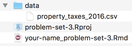
In the end, your project folder should be structured like this:Make sure your .Rmd file is not inside the data folder.

Completing the assignment

1. Ensure that you have your new problem-set-3 project open in RStudio. Open the .Rmd file from the “Files” panel in RStudio and follow the instructions there for the rest of the problem set.

2. Where appropriate, delete the questions I provided and rewrite the text to be more narrative. You can leave all my text for the section called “Basic Regression 1”, since that’s a complete example that you can follow and that you probably want to keep for future reference.

3. Knit the .Rmd as a Word documentOr PDF if you’ve installed tinytex.
   
   when you’re done and submit it via Learning Suite.